Plotting

nctoolkit provides automatic plotting of netCDF data in a similar way to the command line tool ncview.

If you have a dataset, simply use the plot method to create an interactive plot that matches the data type.

We can illustate this using a sea surface temperature dataset available here.

Let’s start by calculating mean sea surface temperature for the year 2000 and plotting it:

import nctoolkit as nc
ff =  "sst.mon.mean.nc"
ds = nc.open_data(ff)
ds.subset(year = 2000)
ds.plot()

visualization_plot1

We might be interested in the zonal mean. nctoolkit can automatically plot this easily:

ff =  "sst.mon.mean.nc"
ds = nc.open_data(ff)
ds.subset(year = 2000)
ds.tmean()
ds.zonal_mean()
ds.plot()

visualization_plot2

nctoolkit can also easily handle heat maps. So, we can easily plot the change in zonal mean over time:

ff =  "sst.mon.mean.nc"
ds = nc.open_data(ff)
ds.zonal_mean()
ds.annual_anomaly(baseline = [1850, 1869], window = 20)gg
ds.plot()

visualization_plot3

In a similar vein, it can automatically handle time series. Below we plot a time series of global mean sea surface temperature since 1850:

ff =  "sst.mon.mean.nc"
ds = nc.open_data(ff)
ds.spatial_mean()
ds.plot()

visualization_plot4

Publication quality plots

The ability to produce plots that are at or close to publication quality was introduced in version 0.9.2 in nctoolkit. This is carried out using the pub_plot method, and is designed to quickly produce a plot that is suitable for a publication or presentation.

ff =  "sst.mon.mean.nc"
ds = nc.open_data(ff)
ds.tmean()
ds.pub_plot()

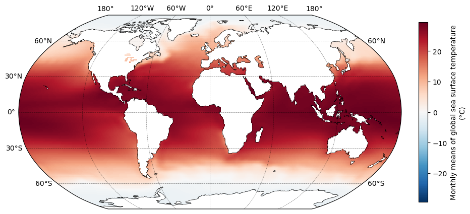
Currently, pub_plot is restricted to work with regular lon/lat grids. A limited number of modifications can be made, such as changes to the colour scale. Over-time this will become a fully featured method.

Plotting internals

Plotting is carried out using the ncplot package. ncplot will look at the dataset and identify a suitable plotting method. This is carried out internally using hvplot. If you come across any errors, please raise an issue here.

This is a package that aims to deliver plotting for rapid exploratory analysis, and therefore it does not offer a large number of customizations. However, because it is built on hvplot, you can use most of the customization options available in hvplot, which are detailed here. Arguments such as title, logz and clim can be passed to plot and will be automatically passed to the hvplot method used .